

When exporting the Activity Table from Primavera P6 to Excel, it can be difficult to visually distinguish between different WBS (Work Breakdown Structure) levels.
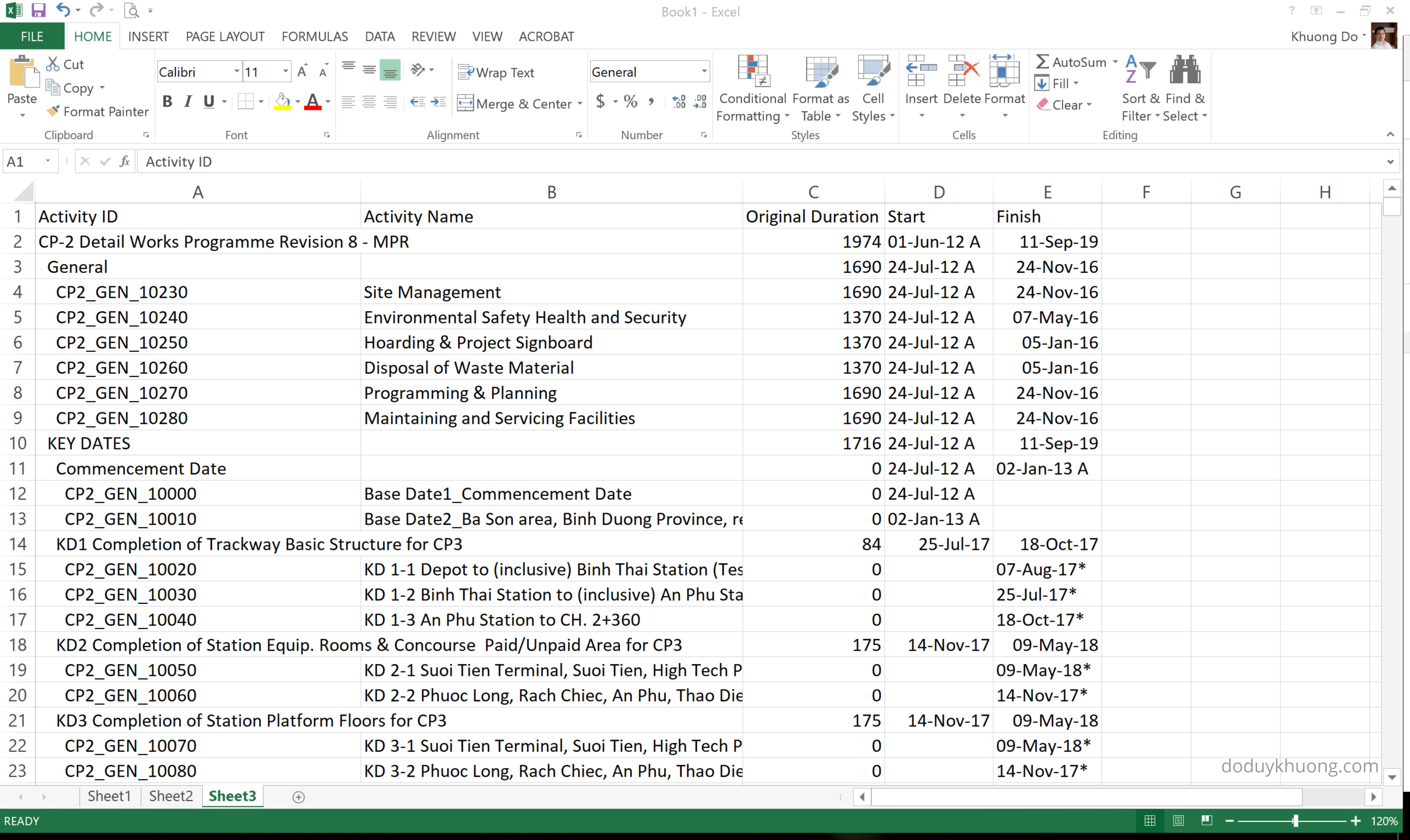
In this guide, I’ll show you how to automatically color-code WBS levels in Excel, making your report easier to read—similar to how it appears in P6.
Step 1: Add the WBS Level Column
First, follow this article to insert the “WBS Level” column into your Excel sheet:

Step 2: Apply Conditional Formatting
Now let’s apply color formatting based on WBS levels:
1. Go to Home > Conditional Formatting > Manage Rules.

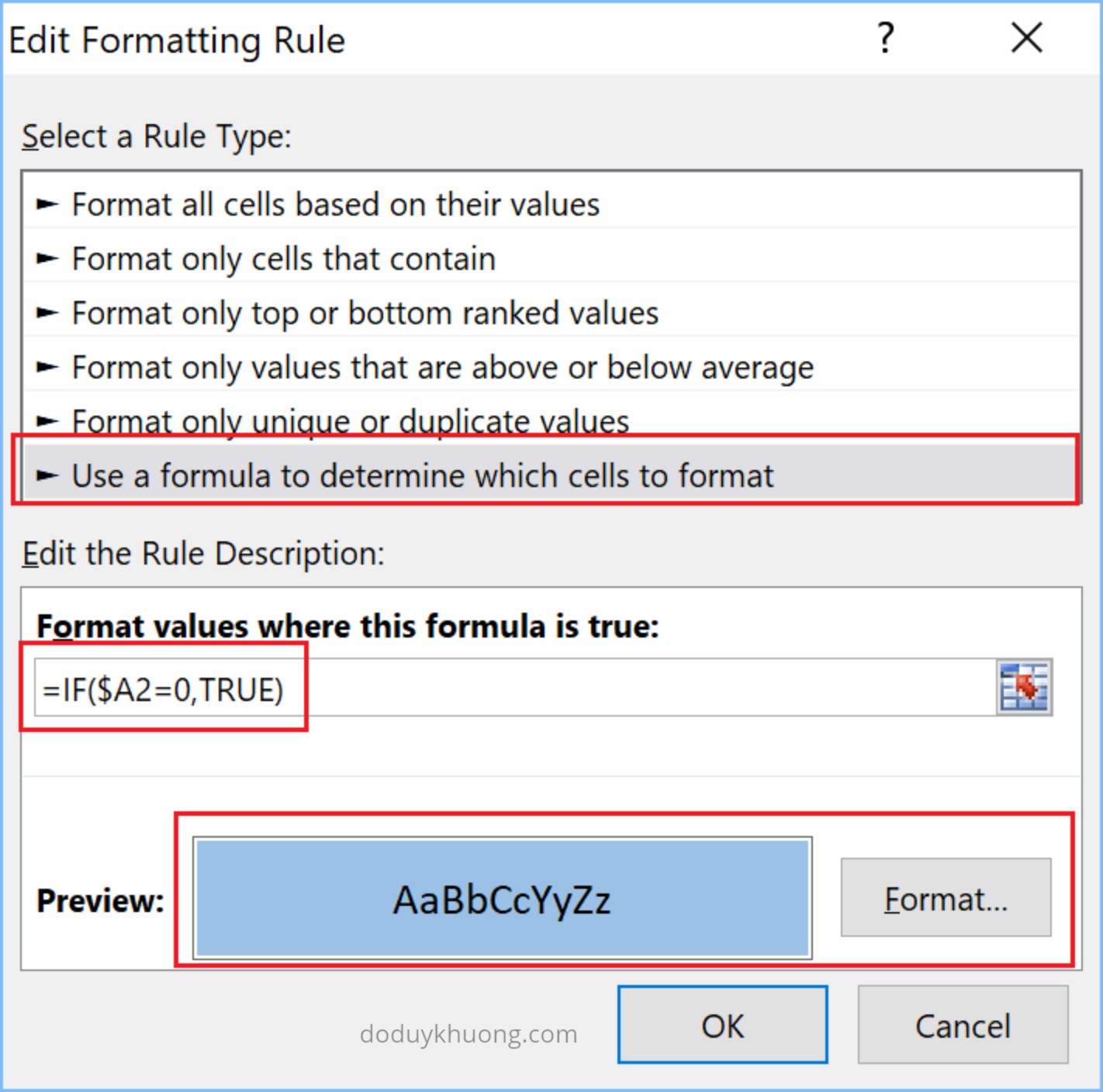
2. Click New Rule, then select “Use a formula to determine which cells to format.”
3. In the formula box enter : =IF($A2=0,TRUE)
4. Choose a color for WBS Level 0 (e.g., green), then click OK.
5. In the Applies to box, click the arrow icon and select the range of cells you want to format (ideally, the entire activity table).
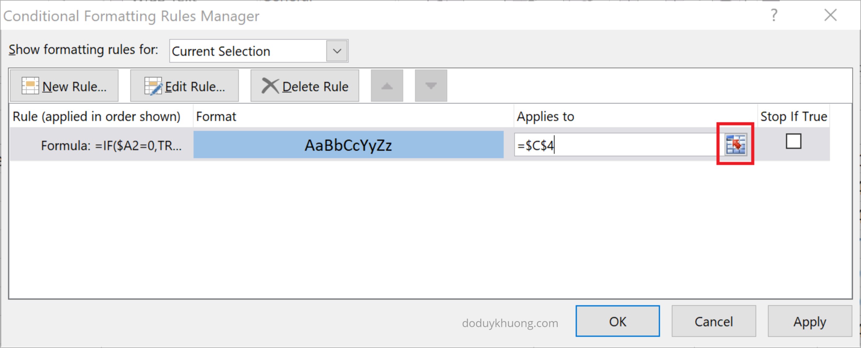

6. Click OK again to apply the rule.
Now every WBS Level 0 will have green color.

Step 3: Repeat for Other WBS Levels
Repeat the process above for other WBS levels (1, 2, 3, etc.). Assign a different color to each level to make the hierarchy visually clear.

Final Result
Once all rules are applied, your Excel report will be color-coded by WBS level—making it much easier to read and analyze, just like in Primavera P6.


i iam doing this but i face problem such after adding conditional formatting formula i dnt c any change
LikeLike
Hi there,
Kindly check your formula carefully. It’s very easy to have a mistake.
LikeLike
Thank you very much, it worked out very well. Keep up the good work.
LikeLiked by 1 person